Why your OpenTelemetry trace shows nothing useful when the CPU is doing all the work — a CP-SAT case study
I run a small production optimization service. It’s not large — a single FastAPI container exposing eleven solver endpoints over REST and MCP, backed by Google OR-Tools CP-SAT, deployed on Railway. It’s mine: I built it, I maintain it, I pay the bill. The public dashboard is live and the source is open on GitHub.
I added OpenTelemetry distributed tracing to it months ago. FastAPIInstrumentor from the opentelemetry-instrumentation package, a BatchSpanProcessor, an OTLP/HTTP exporter pointing to Grafana Cloud Tempo. Five lines of configuration. It worked. Spans appeared. The vendor dashboard showed me green bars. By the standard checklist — “we have tracing” — the service was observable.
And then I ran a load test.
The first call hit POST /optimize_routing. The trace appeared in Tempo within seconds. The total request took 7 milliseconds. I clicked into the trace to see what those 7 milliseconds had been spent on.
This is what I saw.
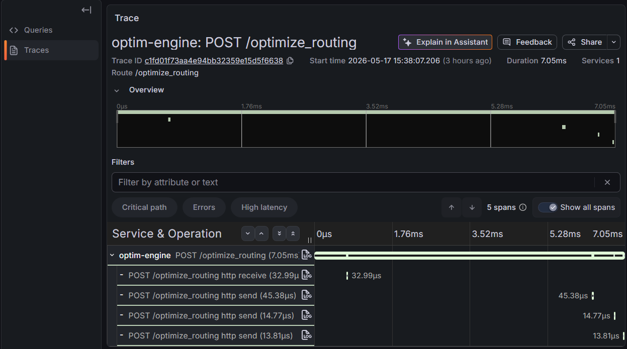
Five spans. One root for the FastAPI handler. Four children, all generated automatically: http receive (32 µs), http send (45 µs), http send (15 µs), http send (14 µs). Total measured time across the children: 106 microseconds out of a 7-millisecond request. The remaining 6.9 milliseconds — the actual work the service did — were nowhere in the trace. They were inside the root span as an opaque interval.
This is the problem I want to write about, because I think it’s a category of failure that doesn’t get named clearly enough. OpenTelemetry, configured the standard way, is a tool that watches the edges of your application. It watches HTTP frames being received and written. It watches database queries fired through instrumented drivers. It watches outbound calls to other services through HTTP clients. What it does not watch, by default, is the CPU work that happens between those edges. And for a class of services — solvers, simulators, ML inference, batch transforms, anything I’ll call compute-bound services in the rest of this piece — the CPU work between the edges is the whole point.
If your service receives a request, talks to a database, and returns a response, OTel-by-default tells you almost everything you need: how long the request spent in the framework, how long in the database, how long going back out. The black box in the middle is small.
If your service receives a request and then runs a constraint solver for fifteen seconds, OTel-by-default tells you that the request took fifteen seconds, and nothing else. The black box in the middle is everything.
That gap is what this post is about. I’ll show you what happens when you push past the default configuration, what the trace actually looks like when you do, and what conceptual frame I think helps when you’re working on services in this category.
The setup that produces the gap
Let me be specific about what “auto-instrumentation” actually instruments, because the failure mode I just showed isn’t a bug. It’s a logical consequence of what auto-instrumentation libraries are designed to do.
FastAPIInstrumentor.instrument_app(app) wraps the ASGI middleware chain. It opens a span when a request arrives and closes it when the response is sent. As part of that, the ASGI protocol’s receive and send events become child spans, because ASGI is asynchronous and those events are the natural framework-level units. So you get one span for the handler and a few sub-spans for the ASGI plumbing.
That’s it. There’s no hook in this instrumentation for your business logic. There isn’t supposed to be. The library doesn’t know what your handler does. It can’t. The instrumentation is correct — it accurately reports what the framework did. It just happens to report only what the framework did.
If your handler delegates to a database, the psycopg2 or asyncpg or sqlalchemy instrumentation will create child spans for the queries. If your handler delegates to HTTP, the httpx or requests instrumentation will create child spans for the outbound calls. Both of those are traversals — they cross a process boundary, and OpenTelemetry’s instrumentation ecosystem is built around crossings.
A CP-SAT solver doesn’t cross a process boundary. It allocates memory inside Python, builds a constraint model, hands it to a C++ library linked into the same process, blocks until the solver returns, reads the solution out, and returns. No HTTP. No database. No queue. From OpenTelemetry’s framework-level perspective, it’s a function call. Function calls aren’t traversals. So nothing gets traced.
The same shape applies to a long list of things people actually build:
- An LLM inference server doing a forward pass against a local model file
- A batch image transformer running OpenCV operations in-process
- A geospatial routing engine running Dijkstra on a loaded graph
- A risk simulation running ten thousand Monte Carlo iterations
- A genetic algorithm doing crossover for a thousand generations
- A regex on a multi-megabyte input that takes seconds to backtrack
For all of these, the work that defines the service is precisely the part OTel-by-default cannot see.
What you actually want to see
Before I show the fix, let me say what I wanted out of the trace, because I think articulating it sharpens what’s wrong with the default.
For an optimize_routing request, the work decomposes naturally into three phases:
-
Build the model. Take the JSON request, parse it into Pydantic objects, compute a distance matrix from coordinates, create the OR-Tools
RoutingModelandRoutingIndexManager, register the callbacks, add the capacity and time-window dimensions, configure the search strategy. This is data structure work. It’s measurable and predictable: a 4-location problem builds in low milliseconds, a 200-location problem in tens. -
Solve. Call
routing.SolveWithParameters(search_params). This blocks until the solver returns either a solution or a timeout. It runs C++ inside the same process. It’s the part where CPU disappears. -
Extract the solution. Walk the solver’s output, build the response objects with route stops, compute aggregate metrics. Predictable: linear in the number of stops.
When I look at a trace, I want to see those three intervals as distinct spans. I want to know whether a 15-second request was 14.9 seconds of solver, or 200 ms of solver and the rest in a bug somewhere in the post-processing. I want to know whether a 4-location problem that’s running slow is slow because the matrix construction has gone quadratic, or because the time-window constraints have become infeasible and the solver is grinding.
The default trace cannot tell me any of that. It tells me “request took 7 ms” and then 99% of the data is missing.
The fix is twenty lines
The fix isn’t conceptually hard. OpenTelemetry exposes a Tracer API that lets you create spans manually, as context managers. The whole library is built so that any code you put inside a with tracer.start_as_current_span("name"): block becomes a named, timed span in the trace tree.
In routing/engine.py, I wrapped the solve_routing function body with one outer span (solve_routing) and three inner spans (build_model, cp_sat_solve, extract_solution). I also added a handful of attributes — optim.num_locations, optim.num_vehicles, optim.solver_status_code — so traces are filterable in Tempo by the shape of the input.
The structure is roughly this, abbreviated for the post:
from api.observability import get_tracer

tracer = get_tracer(__name__)


def solve_routing(request: RoutingRequest) -> RoutingResponse:
    t0 = time.time()
    with tracer.start_as_current_span("solve_routing") as root_span:
        root_span.set_attribute("optim.num_locations", len(request.locations))
        root_span.set_attribute("optim.num_vehicles", len(request.vehicles))
        root_span.set_attribute("optim.objective", str(request.objective))

        try:
            with tracer.start_as_current_span("build_model") as build_span:
                # ... parse, distance matrix, RoutingModel, callbacks,
                # ... dimensions, capacities, search parameters
                build_span.set_attribute("optim.matrix_size", n * n)

            with tracer.start_as_current_span("cp_sat_solve") as solve_span:
                solution = routing.SolveWithParameters(search_params)
                solve_span.set_attribute("optim.solver_status_code", routing.status())
                solve_span.set_attribute("optim.solution_found", solution is not None)

            with tracer.start_as_current_span("extract_solution") as extract_span:
                # ... walk solver output, build response
                extract_span.set_attribute("optim.vehicles_used", num_used)

            return response

        except Exception as e:
            root_span.set_attribute("optim.status", "ERROR")
            root_span.record_exception(e)
            raise
Two real engineering points worth noting in this diff, beyond the obvious.
One, the inner spans are nested inside the outer solve_routing span, not siblings of it. This matters because Tempo lets you query the trace tree, and proper nesting makes queries like “show me all cp_sat_solve spans where the parent solve_routing had optim.num_locations > 100” possible. Flat spans destroy that ability.
Two, the attributes use a custom prefix (optim.*) instead of trying to reuse OpenTelemetry semantic conventions. The semantic conventions are great for HTTP, database, and queue work; they don’t have anything to say about “number of variables in a constraint model”. For domain-specific signals, a custom namespace is honest. Don’t pretend your solver attributes are HTTP attributes just because the conventions don’t cover your domain.
The diff was about ninety lines of code plus reindentation, committed with the message feat(routing): add manual OTel sub-spans for fine-grained CP-SAT observability. It deployed on Railway in two minutes.
The trace after
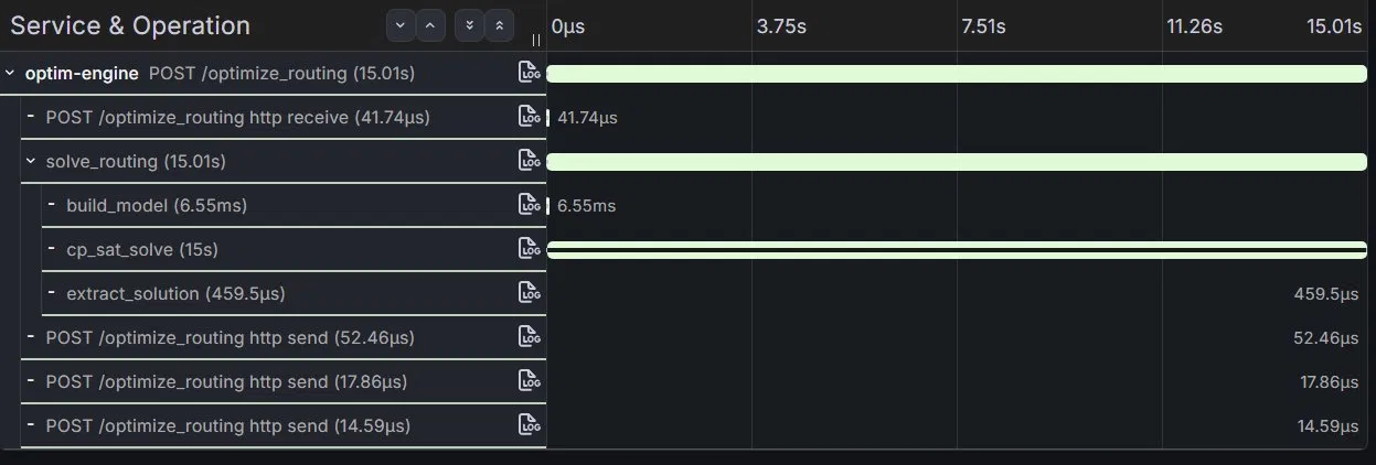
This is the same endpoint, called with a similar but slightly larger problem (4 locations, 1 truck, 24-hour time windows). The total request took 15.01 seconds — the routing solver with GUIDED_LOCAL_SEARCH keeps searching for improvements until the time budget is exhausted, even after finding an optimal solution, which is by design for problems where optimality isn’t provable from the structure.
Read it from the bottom up:
POST /optimize_routingtotal: 15.01 shttp receive(request body): 41.74 µssolve_routing(the manual root): 15.01 sbuild_model: 6.55 mscp_sat_solve: 15.00 sextract_solution: 459.5 µs
http send× 3 (response chunks): 85 µs total
The signal is now unambiguous. 99.97% of the request time was spent inside the CP-SAT solver. Model construction took 6.55 milliseconds — fast and fine. Solution extraction took half a millisecond — fast and fine. Everything else is rounding error.
If this request had instead been slow because the distance matrix construction had gone quadratic for some reason — a bug I’ve actually written in earlier iterations of this service — the trace would have showed build_model at hundreds of milliseconds or seconds, and cp_sat_solve at its expected value. That diagnostic, which is impossible from the auto-instrumented trace alone, is now a single click.
The same holds for the inverse failure mode. If a request times out and I see cp_sat_solve at exactly the max_solve_time_seconds value with no solution, I know the solver hit its budget. If cp_sat_solve is short but the request is slow, the bug is in my post-processing. The trace tells me which it is.
The general shape of the lesson
I think the framing that makes this useful beyond OptimEngine is to separate two questions that the words “observability” and “tracing” tend to blur.
Question one: where is this service spending wall-clock time? Auto-instrumentation of frameworks (FastAPI, gRPC, ASGI) and traversals (HTTP clients, database drivers, queue clients) answers this question well for services where most of the wall-clock time is in framework or traversal work. CRUD APIs, gateway services, orchestration layers — for these, the default configuration is genuinely sufficient. The story is in the edges.
Question two: what is this service actually doing during the time it has? For compute-bound services, the answer to question one — “spending it in a single uninstrumented function” — is not an answer. The black box has to be opened. Manual span instrumentation is the tool for opening it. Without it, you have a checkmark next to “tracing enabled” and no actual visibility.
The trap is that both questions look the same from a vendor dashboard. Both produce traces. Both populate the latency histogram. The dashboard does not warn you that 99.97% of your wall-clock time is hiding in a span attribute called “duration”.
There’s a useful heuristic for which question you should be asking: look at the leaf spans of an actual trace from your service. Sum their durations. Compare the sum to the duration of the root span. If they’re close, your auto-instrumentation is telling you most of what there is to know. If the leaves account for one percent of the root, you have a black-box service and you should treat manual instrumentation as the default, not the optimization.
For most services I’ve worked on or built, this comes down to a single question asked early: is the body of my request handler dominated by Python control flow that calls a heavy library, or by a sequence of awaited network calls? The first is compute-bound. The second is traversal-bound. They need different observability strategies. Auto-instrumentation alone is right for the second, and silently wrong for the first.
What I’m doing next
I’ve been working on this kind of problem in OptimEngine for months. The CP-SAT solver is one shape of compute-bound workload — it’s CPU-bound, single-threaded inside the C++ core, with very specific cost models around model construction versus search.
The shape I’m working on next is different. An LLM inference engine — llama.cpp, vllm, anything that pulls a model into memory and runs forward passes — is also a compute-bound service. The wall-clock time of a /v1/chat/completions request is mostly inside model.generate(), mostly inside a tight tensor-op loop, mostly inside CUDA kernels if you have a GPU. Auto-instrumentation tells you the request took two seconds. It does not tell you whether those two seconds were prefill, decode, sampling overhead, or — most often — paging because RSS overran. The fix shape is similar to what I described here (manual spans inside the inference path), but with a different set of natural decomposition points: tokens-per-second, time-to-first-token, KV cache state.
I’ve been building a Rust tool called inferscope that approaches the same problem from the other side. Instead of asking the engine to instrument itself, it drives the engine over its HTTP API and correlates per-token timing with the engine’s RSS, CPU, and thread count sampled from /proc on a shared monotonic clock. The two approaches are complementary: manual spans tell you what the engine itself thinks it’s doing; an external profiler tells you what the engine actually costs to run, regardless of what it admits in its own traces.
A later post will go into inferscope’s design. For now, the OptimEngine work above is enough to make the point I came in with: if your service is the workload, then watching the edges isn’t observability. It’s a checkmark.
OptimEngine source: github.com/MicheleCampi/optim-engine. Live dashboard (read-only, no login): the public Grafana. The commit adding the manual sub-spans discussed here is on the main branch with message feat(routing): add manual OTel sub-spans for fine-grained CP-SAT observability.
If you’re working on observability for compute-bound systems in Rust or Python and want to compare notes, I’m at michele.campi@outlook.com. I’m currently open to senior IC roles, remote EU.